Adhesion in an Assembly

In this section we are mainly concerned with tubules so thick that we can treat their curvature elasticity as that of smectic-A liquid crystal.

Figure 2. Cross-section of a lipid tubule on a plane orthogonal to its axis. The thickness h of the tubule is fixed.

Hence, we shall use an elastic free-energy density f_el given by

$$f_{el}:=\frac{K}{2} (\kappa _{1} +\kappa _{2})^{2}+\overline{K}(\kappa _{1}\kappa _{2}),$$ (3)

where $\kappa _{1}$ and $\kappa _{2}$ are the principal curvatures of the local lamella in the structure formed by the lipid layers, and both K and $\overline{K}$ are elastic moduli. For a tubule, the cylindrical symmetry requires one principal curvature to vanish, and so f_el reduces to

$$f_{el}=\frac{K}{2} \kappa ^{2},$$ (4)

where $\kappa$ is the curvature of the local layer in the transverse section.

Lipid molecules are anisotropic, and so also are the layers they make up: the response to an external field is different, depending whether the field is normal to the layer or tangent to it. If we apply a homogeneous magnetic field H=He_zwe can write the total free energy per unit length of a thick tubule as

$$F=\frac{K}{2} \int _{{\cal A}}\kappa ^{2}{\mathrm d}a + \tau ... ...int _{{\cal A}}({\mathbf H}\cdot{\mathbf n})^{2} {\mathrm d}a,$$ (5)

where ${\cal A}$ is the annular section of the tubule, $\tau _{0}$ is the surface tension of its boundary, n the unit vector field directed along the generators, and $\chi _{a}$ the diamagnetic anisotropy of the medium. The functional $\cal F$ is subject to two independent constraints: that on the area A of ${\cal A}$ and that on the thickness h of ${\cal A}$.

All layers in ${\cal A}$ are parallel and equidistant curves. An intrinsic way to describe them is by introducing confocal coordinates, as done in Virga & Fournier [8]. If the outer boundary of ${\cal A}$ is taken as the reference curve c for the texture and it is parametrized by its arc-length s, it is possible to express the free energy (5) as a functional of c:

$$F=4\int _{0} ^{L}\lbrace -\frac{K}{2} \sigma \ln{(1-h\sigma )... ...ma )-\frac{1}{2}H^{2}h\cos^{2}{\vartheta}\rbrace {\mathrm d}s,$$ (6)

where $\vartheta$ is the angle between e_x and the tangent unit vector t to c, $\sigma :=\frac{{\mathrm d}\vartheta}{{\mathrm d}s}$ is the curvature of c, and 4L the length of c. Since

$$A=4hL-h^{2}\pi,$$

the constraint on the area of ${\cal A}$ can equivalently be expressed as a constraint on the length of c.

We seek for solutions symmetric with respect to both coordinate axes, as shown in Figure 2. A way to make the equilibrium problem associated with (6) tractable is by changing F into a functional of the focal curve f of the texture, as in [9] (see Figure 3).

Figure 3. The reference curve c and its focal curve f.

As shown in [10], whenever a functional ${\cal F}_{c}$ of a plane curve c with prescribed length L is given by

$${\cal F}_{c}[\vartheta]:=\int _{0} ^{L}\varphi \left( \varthe... ...\frac{{\mathrm d}\vartheta}{{\mathrm d}s}\right) {\mathrm d}s,$$

it can also be written as a functional of the focal curve f parametrized in its arc-length $\ell$:

$${\cal F}_{f}[\vartheta]:=-\int _{\ell _{0}} ^{\ell _{1}}\varp... ...l \frac{{\mathrm d}\vartheta}{{\mathrm d}\ell}{\mathrm d}\ell,$$ (7)

where the relation

$$\ell =-\frac{1}{\sigma},$$ (8)

has been used. The net advantage of the new functional is that the integrand in (7) depends linearly on $\frac{{\mathrm d}\vartheta}{{\mathrm d}\ell}$. Through a variational analysis, it is possible to obtain the equilibrium equation for the focal curve of a regular arc, that is, an arc of c where neither the curvature nor its first derivative with respect to s vanish:

$$\frac{\partial \varphi}{\partial \sigma}(\vartheta ,\sigma)\sigma = \varphi (\vartheta ,\sigma),$$ (9)

which is subject to the appropriate boundary conditions for $\vartheta$ at the endpoints of the arc.

By using (9), one then obtains the angle $\vartheta$ as a function of $\eta :=\frac{\ell}{h}$ (see [10]):

$$\cos{\vartheta (\eta )}=\sqrt{\rho -\frac{1}{4b}\frac{1}{\eta (\eta +1)}},$$ (10)

where $b:=\frac{\chi _{a}H^{2}h^{2}}{4K}$,while $\rho :=\frac{2\tau}{\chi _{a}H^{2}h}$depends on the multiplier $\tau$ which accounts for the constraint on the length of c. It is worth mentioning that $\tau$ has absorbed the surface tension $\tau _{0}$. It is possible to show that for any choice of L and b there exists a unique value $\rho_{b}$of $\rho$ which gives c the fixed length L. Once $\rho$ has been determined, it is possible to retrace the reference curve c through a geometric construction based on the relation between f and c. Figure 4 shows some examples of regular solutions, for different values of $\frac{A}{2h^{2}}$ and b.

Figure 4. (a,b) Regular solution for A/2h²=10 and $b=7.7\times 10^{-3}$, $b=28.2\times 10^{-3}$, respectively. (c,d) Regular solution for a thinner tubule with A/2h²=10³and $b=1.3\times 10^{-6}$, $b=4.8\times 10^{-6}$, respectively. These latter values are such that the magnetic field has one strength for the pair (a,c), and another one for the pair (b,d), but it is equal for both solutions in one and the same pair.

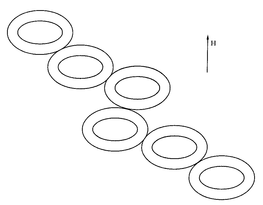
We have just learnt that the external magnetic field can deform a tubule. We now consider an assembly of tubules equal in shape, allowing for mutual adhesion between them. The contact forces and the external ones may compete in establishing the stable equilibrium pattern. Besides the regular solutions just found, we can search for solutions exhibiting flat sides along which any tubule adheres to the adjacent ones. It has been shown in [10] that for every strength of the applied field there is a critical value w_c of the adhesion potential, above which, in the stable configuration of an assembly, each tubule adheres to its neighbours along two opposite flat sides orthogonal to the field, as shown in Figure 5

a) b)

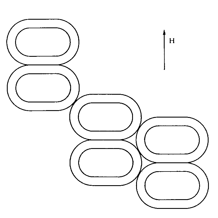
Figure 5. Sketches for an assembly of tubules. In (a) they adhere to one another, whereas in (b) they do not.

When w<w_c, the tubules in a stable assembly do not adhere to one another: they may touch along lines which bear no energy. Figure 6 illustrates the stability diagram corresponding to one value of $\frac{A}{2h^{2}}$. The function g(b) is defined as $g(b):=b(\rho _{b}-1)$.

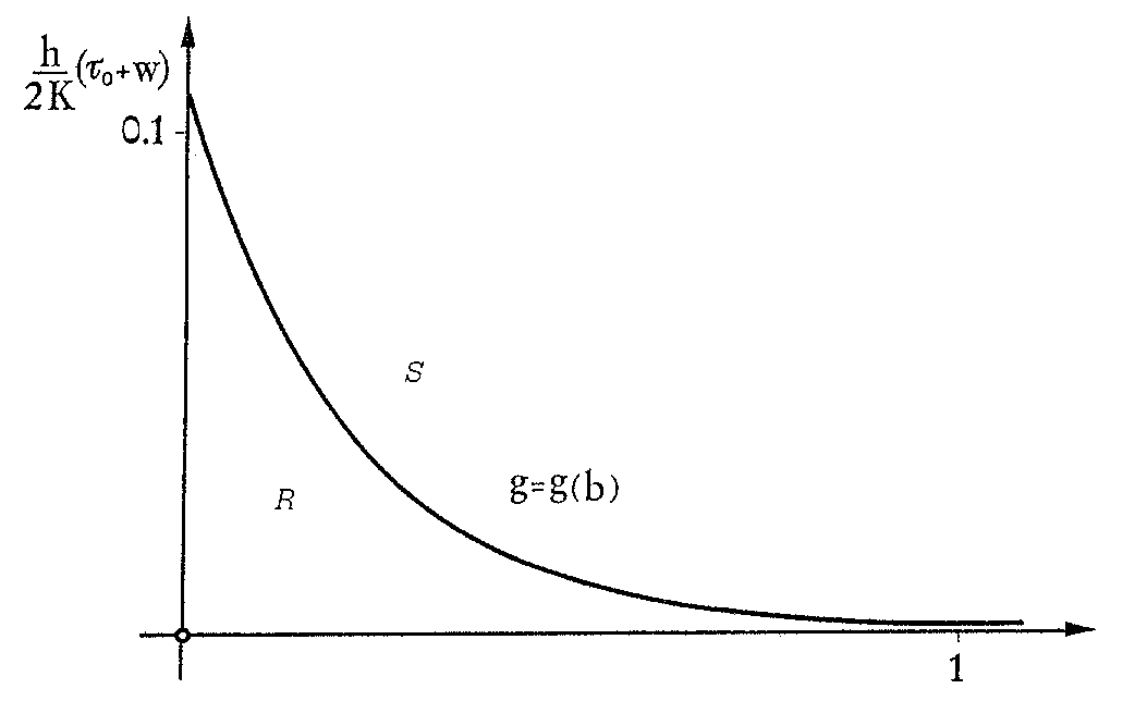
Figure 6. Stability diagram for an assembly of tubules, when A/2h²=5. The regions $\cal R$ and $\cal S$ are separated by the graph of g. The points in $\cal R$and $\cal S$ represent, respectively, regular and singular energy minimizers. In $\cal S$, the tubules adhere to one another.