Adhesive Borders

We have remarked in Section 1 that amphiphilic molecules tend to organize themselves into bilayers, in order to reduce the contact between their hydrophobic tails and water. This contact can be further reduced either when the bilayer is closed, so as to form a vesicle, or when it is not closed, but the molecules along its border $\cal C$ are arranged as in a splay (see Figure 10)

Figure 10. Sketch of a border.

Of course, the molecular splay has an energetic cost: according to Helfrich [13], it can be given the simple form

$${\mathcal{F}}_{\ell}[{\mathcal{C}}]:=\gamma L(\mathcal{C}),$$ (17)

where $\gamma$ is a positive constitutive parameter which represents a line tension. Here we are primarily concerned with the appropriate equilibrium conditions along a border, which differ from those already obtained for the points where the principal curvatures of a vesicle suffer a jump, as do the admissible deformations of the membrane. Along a border, a fluid membrane can only glide on the wall, and so its displacements must always be tangent to the wall (see Figure 11).

Figure 11. An open fluid membrane that adheres to a rigid wall. $\mathcal{S}^{*}$ is the free membrane and $\mathcal{S}_{*}$ the adhering one; $\mathcal{C}_{*}$ is the adhering contour, and $\mathcal{C}$the adhesive border of ${\mathcal S}$. The principal curvatures of the membrane may jump along $\mathcal{C}_{*}$. The unit normal $\mbox{\boldmath$\nu$ }_{*}$ to $\mathcal{S}_{*}$ is the same as the unit normal to the wall.

On the other hand, an open membrane could also adhere to the wall along the border and be completely detached elsewhere (see Figure 12).

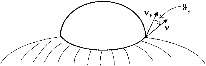
Figure 12. An open fluid membrane in contact with a rigid wall only along its border $\mathcal{C}$. Here, there is neither an adhering contour nor an adhering membrane. The angle $\vartheta_{c}$ that the normal to ${\mathcal S}$ makes with the normal to the wall along the border of the membrane is the contact angle.

In this case, the admissible displacements of the border can no longer be tangent to the membrane.

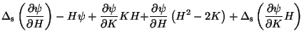
Starting from (1) and (2), one can derive a general equilibrium equation for a free membrane, which reduces to Ou-Yang and Helfrich's [14] when their special energy functional is used. This equation was obtained in [15] through an intrinsic method, that is, which does not resort to any specific system of coordinates to represent the equilibrium shape of the membrane:

 

$$\Delta_{\mathrm{s}}\left( \frac{\partial\psi}{\partial H}\right) ... ...}-2K\right) +\Delta_{\mathrm{s}}\left( \frac{\partial\psi }{\partial K}H\right)$$

$$-\mathrm{div}_{\mathrm{s}}\left[ \left( \nabla_{\mathrm{s}}\mbox{... ...ta_{\mathrm{s}}\mbox{\boldmath$\nu$ }\cdot\mbox{\boldmath$\nu$ }% -\lambda H=0.$$ (18)

In (18) $\Delta _{s}$, div _s and $\nabla_{s}$ denote, respectively the surface Laplacian, the surface divergence, and the surface gradient; $\mbox{\boldmath$\nu$ }$ is the unit normal vector to the membrane and $\lambda$ is a Lagrange multiplier which accounts for the inextensibility of the membrane. Moreover, $H:=\frac{\sigma _{1} +\sigma _{2}}{2}$ is the mean curvature and $K:=\sigma _{1}\sigma _{2}$ he Gaussian curvature.

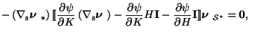
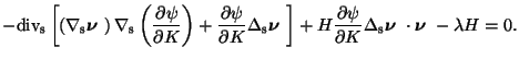
Besides this equation, an open membrane in contact with a wall must also satisfy other equilibrium conditions on both its possible adhering contours and its adhesive borders. The former equilibrium condition reads as

 

$$[\hspace{-0.05cm}[\psi]\hspace{-0.05cm}]\mbox{\boldmath$\nu$ }_{\... ...rtial K}\mathbf{I}]\hspace{-0.05cm}]\mbox{\boldmath$\nu$ }% _{\mathcal{S}^{*}}-$$

$$-\left( \nabla_{\mathrm{s}}\mbox{\boldmath$\nu$ }_{*}\right) [\hs... ...}_{\mathcal{S}^{*}% }=\mathbf{0,}$$ (19)

where $\mbox{\boldmath$\nu$ }_{\mathcal{S}^{*}}$ is the outer normal to ${\mathcal S}$ along the adhering contour $\mathcal{C}_{*}$, as shown in Figure 11. Equation (19) restricts the possible jumps of the principal curvatures of the membrane across the adhering contour $\mathcal{C}_{*}$ and is a further extension of the condition found by Seifert and Lipowsky [6].

On an adhesive border $\cal C$, when the membrane is everywhere tangent to the wall (see Figure 11) the equilibrium condition reads as

$$\psi+\lambda-\gamma\kappa_{\mathrm{g}}=0\qquad\mathrm{on\ }\mathcal{C}% , %$$ (20)

where the line tension $\gamma$ is defined as in (17), $\lambda$ is the Lagrange multiplier associated with the constraint on the total area of the membrane, while $\kappa_{\mathrm{g}}$ is the geodesic curvature of $\mathcal{C}$. On the contrary, when the membrane is not tangent to the wall along the border, as in Figure 12, $\mbox{\boldmath$\nu$ }$ and $\mbox{\boldmath$\nu$ }_{*}$ may differ. If we call $\vartheta_{c}$the contact angle $\vartheta$ between the membrane and the wall (see Figure 12), equilibrium conditions along the adhesive border can be given the form

$$\frac{\partial\psi}{\partial H}=\kappa_{\mathrm{n}}\frac{\partial\psi }{\partial K}\ , %$$ (21)

where $\kappa_{\mathrm{n}}$ is the normal curvature of $\mathcal{C}$ and

$$\tan\vartheta_{c}=\frac{\psi+\lambda-\gamma\kappa_{\mathrm{g}... ...{g}}\frac{\partial\psi}{\partial K}\right) \cdot\mathbf{t}}, %$$ (22)

where $\tau_{\mathrm{g}}$ is the geodesic torsion of $\mathcal{C}$.

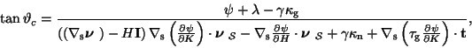
When axisymmetric membranes are considered and $\psi$ is taken as

$$\psi=\frac{k_{b}}{2}H^{2}+k_{G}K, %$$ (23)

where k_G is the Gaussian elasticity of the membrane, equations (21) and (22) become

$$(k_{b}+k_{G})\sigma_{p}+k_{b}\sigma_{m}=0, %$$ (24)

$$\tan\vartheta_{c}=-\frac{\psi+\lambda-\gamma\kappa_{\mathrm{g... ...{p}+\sigma_{m})\cdot\mbox{\boldmath$\nu$ }% _{\mathcal{S}}}, %$$ (25)

where $\sigma_{p}$ and $\sigma_{m}$ are the principal curvatures of the membrane along $\mathcal{C}$, while $\mbox{\boldmath$\nu$ }_{\mathcal{S}}$ is the unit outer normal to $\mathcal{C}$, tangent to ${\mathcal S}$(see Figure 12).

As an application of (20), we have studied in [15] the stability for an adhesive border, when the adhesive body is a cone, as illustrated in Figures 13a & 13b

a) b)

Figure 13. The adhesion of a membrane to two axisymmetric bodies: the cones in (a) and (b) are reverse to one another, but with the same amplitude $2\alpha$. The equilibrium of the border $\mathcal{C}$ is unstable for the former and stable for the latter.

The analysis of (20) allows us to conclude that the equilibrium configuration shown in Figure 13a is unstable, whereas that shown in Figure 13b is stable.